Marginal Loss Factors: Will someone please repeal the laws of physics?

Like waiting for exam results, generators await the Australian Energy Market Operator’s (AEMO) March release of draft Marginal Loss Factors (MLFs) with excitement and dread[1]. This arcane document has big effects upon the profitability of power stations for the coming year.

Like previous years, last Friday’s release contained some bad news for some generators. Remote solar and wind generators had some big write downs that even drew mainstream media attention[2] and a call from the Clean Energy Council (CEC) for a change in approach[3].

However these MLF changes were entirely to be expected because AEMO’s numbers are simply an expression of the laws of physics, which are awfully difficult to amend. We take a look at MLFs, drawing upon an excellent reference document published by AEMO[4].

What are electrical losses?

Whilst high voltage conductors transport electrical energy wonderfully efficiently, sadly they still lose some of it along the way in the form of heat. Typically around 10 per cent of the energy that leaves a power station never makes it to a consumer.

Figure 1: Losses across a transmission line

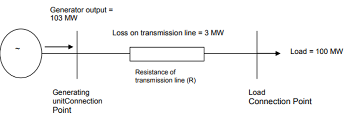Source: AEMO

We hopefully all remember from high school some formula about “I squared R”. This means losses in a line increase with the resistance of the line, and with the square of the current. As power is proportional to current, losses increase with the square of the power transferred on a line.

Understanding losses is a key element of planning networks and locating generation. And also when operating the power system – it is a simple fact that extra power must be generated to cover losses, and this generation must be paid for.

Fortunately, a power system’s loss characteristics can be accurately calculated in a loadflow model, a tool that AEMO uses to calculate MLFs. MLFs are the way these losses can be expressed to participants in an electricity market, driving them to collectively manage losses in the same way as a central operator would.

How do we represent them in an electricity market?

There are three key features to understand the basic premise of loss factors in the National Electricity Market (NEM):

• The parabolic loss characteristic from the square term above, (a law of physics),
• The marginal pricing approach used in all electricity markets (a law of economics), and
• The regional settlement mechanism employed in the NEM (a design choice).

Figure 2: Marginal versus Average Loss Factors

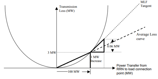Source: AEMO

In Figure 1’s simple transmission line, the total losses were 3 per cent. However, in Figure 2, because losses increase with the square of the power transferred, when the load increases by 1MW, the generator will need to increase output by 1.06MW, i.e. the marginal losses are actually 6 per cent.

Figure 3: Marginal (1MW) increase in load

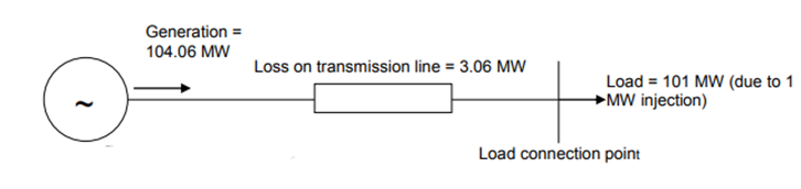Source: AEMO

Electricity markets, like all markets, settle their prices at the intersection of the supply and demand curves. This is called a “common-clearing price”. It means the price for all production and consumption is set by the marginal value of trade, i.e. the cost of meeting the next increment of demand.

This means that if the generator’s marginal price is $100, the customer’s marginal price should be $106. If there was a competing generator at the load point whose marginal price was $105, this would be cheaper to run than the remote $100 generator, and AEMO would dispatch it first. This results in the most efficient dispatch possible, and is the basis for loss price differences across the NEM, which the MLF process supports.

Interestingly, because marginal losses (6 per cent in the example above) are larger than average losses (3 per cent), settling prices based on the marginal losses leads to AEMO recovering, in total, more from customers than it needs to pay generators. In the NEM this is called the intra-regional settlement surplus (IRSS) and is refunded to customers via an offset to their network rates.

Generators sometimes suggest that the IRSS should instead be directed their way to offset the pain of loss factors[5]. However this would run contrary to the marginal pricing upon which electricity markets are based.

The next question is how to geographically present the losses of transmission lines. Many markets, such as those in the US, Singapore and New Zealand use nodal pricing. In these markets the dispatch engine incorporates a real-time loadflow and the price of every point on the transmission system is continuously adjusted for the marginal losses between it and whatever bid is setting price at the moment of dispatch.

The NEM however chose to use regional pricing with prices based on a hub and spoke model. Large geographical regions are created, each having a regional reference node (RRN) arbitrarily selected from the transmission system, which becomes the hub and given a fixed MLF of 1.00.

All of the other nodes are then described as spokes around this hub, and given an MLF in reference to it- see Figure 4. Generator spokes will get MLFs below 1.00, and Customer spokes above 1.00. Generation or load at each point is then settled at the RRN price times the local MLF.

The selection of the RRN should not matter as it becomes mathematically redundant to the calculations. Consider figure 3 above: assuming all else is equal, it does not matter which end is nominated to be the RRN, the generator and the load will still be settled the same.

The network between the RRNs is represented as an interconnector. Despite public perception, an interconnector is really just a mathematical concept of the dispatch engine rather than a dedicated physical asset. Between the RRNs AEMO uses Inter-Regional Marginal Loss Factors.

Figure 4: NEM Regional pricing and the hub and spoke model

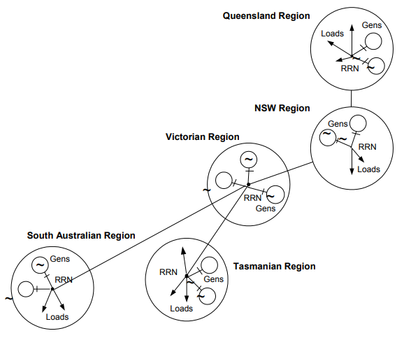
Source: AEMO

How are they calculated

As discussed above, nodal markets inherently adjust continuously for their losses. Similarly, the NEM’s inter-regional loss factors change dynamically based on conditions. AEMO has pre-calculated interconnectors’ loss parabolas so that the dispatch engine can estimate the their marginal losses, given current dispatch, every five minutes.

However the NEM applies static MLFs intra-regionally as a simplification. Each generator and load point is given an MLF that applies for an entire financial year. These are what AEMO reveals every March.

Static MLFs are calculated by running a loadflow on the expected dispatch of every half hour of the upcoming year, thereby producing 17,520 MLFs for every transmission node. These MLFs are then volume-weighted by the generation or load at that point to get a static average.

This gives, over time, a broadly correct signal from a financial point of view and is appropriate for investment signals. However the simplification does lead to some inaccuracy in five minute pricing and dispatch. For example the static loss factor of a highly variable generator like a windfarm will tend to over-penalise it during light wind periods whilst under-penalising during high wind.

The possibility of moving to more dynamic intra-regional loss factors was once reviewed by AEMO’s predecessor, NEMMCO, who concluded the dispatch accuracy was not worth the additional complexity. This was however before the emergence of variable generation.

Whilst it would improve five minute pricing accuracy, given the volume weighting behind static loss factors, the long-term revenue consequences of changing from static to dynamic loss factors would be minor.

Why do they change?

A quick review of this year’s draft loss factors shows most conventional generators enjoying fairly stable MLFs, whilst many solar and wind generators are taking haircuts. Whilst providing a wonderful basis for a conspiracy theory, this is in prosaic reality an expected outcome of a changing power system subject to the laws of physics. Solar and wind generators are flocking to areas that were previously small rural load centres, connected to the RRN by long, high resistance lines.

Broken Hill is connected to Buronga 300km away by an extreme example of a long skinny line. As a remote small load centre its loss factor was historically well above 1. The building of two large renewable projects there has caused one of these projects’ MLF to now fall to only 0.799.

In the Broken Hill case the projects were developed by one party, so they could predict this outcome. However it is also true that loss factors of some incumbent plants have been significantly affected by the rapid connections of neighbouring competitors. Similar to congestion risk, this a risk that generators face in the NEM’s open-access network regime.

The Renewable Energy Target Scheme

The granting of Large Generator Certificates (LGCs) are also adjusted by the MLF. The Renewable Energy Target (RET) scheme’s designers drew upon the NEM’s existing mechanism to reward renewable generators located in less lossy areas. However this design does create strange outcomes, as, unlike the settlement of energy, the RRN location is not mathematically redundant.

For example, when the snowy region existed, LGCs created at its RRN, Murray power station, had no adjustment. But following the abolition of the region, LGCs created there are now discounted by over 6 per cent, despite there having been no physical change. And the use of Georgetown, rather than Hobart, as RRN provides Tasmanian generators a couple of extra per cent LGC creation.

Note these anomalies are an outcome of the design of the RET, not the MLF design itself which works well for its intended purpose of signalling the marginal value of electricity. Inevitable issues arose because the RET piggy-backed on a loss factor design never intended for this purpose.

What options do participants have to manage them?

Before investing in a plant, it is necessary to contemplate the loss factor risks carefully. Expert engineering consultants can run loadflows similar to that of AEMO to predict MLFs. These should include scenarios where neighbouring plants connect.

Having invested, there is not much a generator can do to insure itself, as there is no natural counter-party with an offsetting risk. Network investment can improve MLFs, but making a significant dent in losses usually requires very large augmentations. Losses are an allowable benefit in network augmentation justification, but tend to be a second-order benefit. 

So it’s really an issue that needs to be carefully considered before investment – a developer should favour locations with low resistance between the connection point and large load centres. Take for example the Bald Hills, Toora and Wonthaggi wind farms, located in Victoria’s Gippsland region. These benefit in part from the emerging surplus of transmission between the Latrobe Valley and Melbourne and enjoy loss factors close to 1.00.

Conclusion

Losses in a transmission network are a natural physical phenomenon and all electricity markets must find ways of:

• dispatching additional generation to supply them,
• paying for the additional generation, and
• maintaining the correct marginal incentives in order to encourage efficient investment and dispatch.

The NEM’s MLFs regime attempts to do all the above three. The regional market design, combined with static yearly loss factors is the result of an initial simplification decision that, as a trade-off, introduced some inaccuracy.  It would be worthwhile re-assessing whether, given the changes in the power system, the trade-off continues to represent the correct balance.

However it should also be noted that greater accuracy is unlikely to bring much joy to those parties who have been affected by adverse MLFs, as there is no reason to expect that greater accuracy would significantly improve their circumstance. The only way to reduce exposure to adverse MLFs is to very carefully assess the likely losses prior to investment. In fact this is exactly what the design of MLFs seeks to encourage.

---

 

[1] AEMO, Draft Marginal Loss Factors: FY 2019-20, March 2019

[2] AFR, Grid anarchy: Wind and solar farms cop haircut from market operator, 13 March 2019

[3] CER, Clean Energy Industry Calls For Urgent Reform to Marginal Loss Factor Arrangements, 8 March 2019

[4] The theory and diagrams in this article draws heavily from AEMO “Treatment of Loss Factors in the NEM” July 2012 available at www.aemo.com.au

[5] See Adani rule change proposal https://www.aemc.gov.au/rule-changes/intra-regional-settlement-residue-reallocation